Wellbores and Deliverability

The "deliverability" of a system is its capacity to deliver gas as a function of pressure. The maximum possible capacity is called the absolute open flow potential (AOF), and reflects what the system could deliver if there were no external losses acting on it; (i.e. if the flowing pressure was equal to zero).

There are several options available in Piper where you can enter well deliverability data, based on the type of gathered data. These are:

Fixed Gas Rate
Test Wellhead Flow Rate/Pressure
Wellhead C and n
Sandface C and n
Transient Deliverability
Profile Deliverability

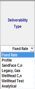
The toggle buttons in the Well Deliverability editor are used to switch between the different options and highlight the necessary input cells (for any selected mode, the non-required cells are blued-out).

On-Stream Date

The date in which a well is to become active in the forecast interval set in the Forecast View tab. A well becomes active on the later of the on-stream date or the first date of the forecast interval.

Note: Although a well can have an on-stream date before the forecast period begins, Piper does not calculate the deliverability of the well for the period before the forecast interval. The well starts producing on the first forecast date if on-stream is set before the forecast date.

If the on-stream date is blank, a well is active the first forecast date.

UNITS: MM/DD/YYYY

DEFAULT: None

Fixed Rate Deliverability

General

This option represents a well that produces at a Fixed Gas Rate irrespective of pipeline, or reservoir pressures. The main purpose for this option is for tuning the system. The introduction of a fixed volume of gas simplifies the tuning process because with a fixed rate option a change in tuning parameters will only affect the flowing pressures in the system. This function is also a very useful option when a volume of gas is being brought into a gathering system but there is no reservoir or deliverability information available for it.

Fixed Rate Wells and Reservoirs

A Fixed Rate well can be connected to a reservoir. The reservoir will deplete, but the well performance will be independent of reservoir depletion.

However, a Fixed Rate well attached to a reservoir in Piper will shut-in. The criteria that determines whether a Fixed Rate well can flow is the static wellhead pressure. Piper will calculate the static wellhead pressure from the provided reservoir pressure and a static gas gradient from the reservoir to surface. If the line pressure exceeds the static wellhead pressure, the Fixed Rate well will be shut-in.

If there are a number of Fixed Rate wells in the model, Piper will shut-in wells with the lowest wellhead static pressure first. The ability of a Fixed Rate well to flow is thus independent of the downstream location of the well.

Profile Deliverability

A profile deliverability well behaves much like a fixed rate well. The rate specified for a profile well is independent of pressure. The difference between a profile well and a fixed rate well is that with a profile well the rate the well flows at is specified on a period-by-period basis.

When the profile well is selected in the Well Deliverability editor, you can either choose from existing profiles, or create a new profile. Note that the same profile can be assigned to more than one well.

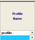
Note that a rate entered in the first row corresponds to the rate in the first forecast period, and so on. If you want the well to begin producing at a later date, the rate data can be entered beginning at a higher row number. Blanks can be left in the prior rows.

Background for Sandface and Wellhead Deliverability

In Piper deliverability can be defined in two locations:

At the Sandface
At the Wellhead

The Sandface Deliverability curve is sometimes referred to as the Inflow Performance Relationship (IPR). The Wellhead Deliverability Curve is sometimes referred to as the Outflow Performance Relationship (OPR). The difference between the Wellhead and the Sandface deliverability is due to the hydrostatic and frictional pressures losses of fluids flowing within the wellbore.

A typical Deliverability plot of both Sandface and Wellhead deliverability is shown below:

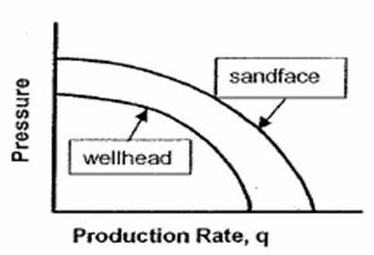
To define the deliverability at the wellhead, a 'Wellhead C,n' well should be chosen. To define deliverability at the sandface, a 'Sandface C,n' well should be chosen. Note that a 'Wellhead C,n' well will not take into account the effect of a wellbore, whereas a 'Sandface C,n' well will account for the effect of the wellbore.

Difference between Wellhead Test and Wellhead C,n Deliverability

The Wellhead Test Deliverability and Wellhead C,n Deliverability are identical in how they model deliverability. The different between the two is that the Wellhead Test deliverability will calculate the C value based on the current test rate and pressure that is entered, while the C, n Deliverability requires that the user enter the C, n values explicitly.

Using Turner or Coleman Correlation with Wellhead Deliverability Wells

Wellhead deliverability wells have, as their names suggests, their deliverability defined at the surface. Therefore, wellbore information is not required and is in general not used. An exception to this rule is when the Turner or Coleman critical liquid lift correlation is turned on and a wellbore has been defined.

In this case Piper will perform a check on the well, using the current well rate and pressure. The rate and pressure are extrapolated down to the end of tubing using the selected pressure loss correlation, and a comparison is made of the velocity of the gas at the end of tubing against the critical velocity required to lift liquids given the selected liquid lift correlation. If the velocity of the gas is less then critical velocity, Piper notify the user and shut the well in.

This provides users with a diagnostic to detect approximately when wells will load up without having to model those wells with the detail of the Sandface C,n or Transient deliverability model.

Note that the above steps are used strictly for determining the ability of a well to lift liquids at EOT, and that the wellbore is not used in any other of the wellhead calculations.

Wellhead Test Deliverability

General

This option allows you to enter a measured Wellhead flow rate and Wellhead flowing pressure from which Piper will calculate the deliverability for the well using the backpressure equation.

The backpressure equation is also governing known as the Rawlins-Schellardt backpressure equation. It is a universal relationship that applies to all gas wells and is independent of reservoir drive. It is generally derived from AOF or Inflow performance testing but can be estimated from current operating conditions if certain assumptions are made. For Wellhead Deliverability the for of the backpressure equation that is used is:

Note that there are two constants that define the deliverability of the well in the backpressure equation; the C and the n. For a Wellhead Test Deliverability the ‘n’ can be specified by the user if it is known or can be estimated. If the Wellhead 'n' is not specified, a default value of 1 will be assumed. A default value of 1 corresponds to very laminar flow, so little in the way of near-wellbore turbulent pressure losses, so it is most appropriate for aging wells or for low deliverability wells.

To perform the calculation of the C value, Piper will take the current reservoir pressure and adjust that pressure with a static gradient to come up with a corresponding static Wellhead Pressure. It will then use that static pressure, along with the current operating rate and pressure, to solve for C.

To use the Wellhead test option in Piper the well must have a reservoir associated with it in the Well Deliverability menu.

Wellhead Test Flow Rate

This is the raw gas flow rate, measured at the wellhead, at the Test Wellhead Flowing Pressure. The program uses these values to calculate the Wellhead "C" and "AOF".

UNITS: MMscfd (103m3/d)

DEFAULT: None

Wellhead Test Flowing Pressure

This is the flowing pressure measured at the wellhead, and corresponding to the Test Wellhead Flow Rate.

UNITS: psia (kPaa)

DEFAULT: None

Wellhead C,n Deliverability

General

This option allows the user to specify the Wellhead "c" and Wellhead "n" as determined from standard AOF/Back Pressure/Deliverability tests.

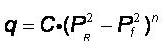
The equation governing the Inflow Performance Relationship is known as the Rawlins-Schellardt backpressure equation. It is a universal relationship that applies to all gas wells and is independent of reservoir drive. It is generally derived from AOF or Inflow performance testing. For Wellhead Deliverability the equation is stated as:

Where:

q = flow rate, MMscfd or 103m3/d
C = constant, MMscfd/(psi2)n or (103m3/d/kPa2)n
n = turbulence of flow, dimensionless
Pts = static wellhead pressure, psi or kPaa
Ptf = flowing wellhead pressure, psi or kPaa

Wellhead, C

The “C” value for a well defines the magnitude of the wells rate response to changes in pressure. Larger C values will correspond to higher deliverability wells. A wellhead C value is sometimes available from a Welltest report. Alternatively, it can be calculated in the same way already described in the section Wellhead Test well Deliverability.

There are no limits on the range of allowed "C" values due to the complicated interaction between C, AOF, n and pressure. Be aware, however, that the system is very sensitive to changes in "C" and that extreme values of "C" can result in extremely large deliverability potentials which can cause system instabilities.

Wellhead, n

The ‘n’ value is a measure of the effect of turbulence in the near-wellbore region on the well’s performance. Values for "n" are valid only between 0.5 and 1.0. A default value of 1 corresponds to very laminar flow, so little in the way of near-wellbore turbulent pressure losses. A value approaching 0.5 would correspond to significant losses due to highly turbulent flow in the near-wellbore region.

Values of n closer to 0.5 are most appropriate for wells that are expected to flow at high drawdowns, or for wells with high deliverability potential. Values approaching 1 are most appropriate for aging wells or for low deliverability wells. Note that while in theory a value of n = 1 should not be possible, standard practice often prescribes an n value of 1 to aging or low deliverability wells that are expected to flow at a low rate.

If, in the Well Deliverability editor, the Wellhead 'n' is not specified, a default value of 1 will be assumed.

Input values less than 0.5 are automatically defaulted to 0.5 upon choosing OK to close the Well Deliverability Editor. Similarly, values greater than 1.0 are automatically defaulted to 1.0.

Transient Deliverability

This deliverability option models a well that produces from a single region or two-region composite reservoir of either finite or infinite dimension.

The distinct features of the Transient Deliverability well type are:

The transient deliverability type will model the early time transient behavior (usually an initial flush production) by accounting for the period before boundary dominated flow is reached.
Once a transient deliverability well ‘sees’ the boundaries of the reservoir, it behaves in much the same manner as a conventional C, n deliverability, with the productivity index for the well defined based on the well parameters that are defined (k, s, Ø, net pay, sw)
The transient deliverability type models only single well pools. Therefore it does not account for effects of interference between wells in the same pool

The deliverability of a transient well is determined by the reservoir/deliverability parameters input in the Transient Well Editor. The Transient Reservoir and its impact on deliverability is discussed in detail in the section Transient Reservoir.

There are two solutions to the diffusivity equation which the transient well model uses to define its deliverability. One solution is for the flow period before the reservoir boundaries have been reached, and the other solution is for the flow period after the boundaries have been reached. At each flow period, the transient deliverability model determines whether the boundaries of the reservoir have been seen, and then applies the appropriate solution. For example, in the case of a single zone, finite radial model, the following analytical models would be used, depending on whether the well has seen the boundaries of the reservoir:

Transient (early-time) Flow:

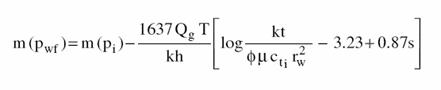
For the late time, Boundary Dominated Flow:

Transient Wells Associated with Wellbores

The transient deliverability model is a deliverability at the sandface and thus it can be associated with a wellbore. When a transient well is associated with a wellbore, pressure losses within the wellbore due to frictional and hydrostatic effects will be accounted for.

Multiphase flow losses can be modeled by specifying a LGR for the transient well and choosing an appropriate multi-phase correlation. Piper will solve to a converged solution that will match the surface conditions to the bottomhole conditions taking into account the appropriate pressure loss in the wellbore.

Transient Wells that Consider Liquid Loading

The Turner or Coleman critical liquid lift correlations can be used with transient wells that have been associated with a wellbore. When the Turner or Coleman correlations have been turned on, the transient well will be tested to determine whether the transient well has the ability to lift liquids.

See the section Liquid Loading wells for details on the loading options.

Analytical Models

Piper allows you to import RTA analytical models and forecast those models forward under the constraints of the gathering system. The analytical models provide better simulation of transient flow behavior then do the traditional steady state models such as the Sandface and Wellhead C and n models. This is an important consideration when dealing with the following situations:

Modeling of early time “flush” production from new wells
Predicting short-term back-out of existing wells when new wells are brought on-stream
Investigating the short term versus long term impact of debottlenecking alternatives, such as adding compression or looping lines

Gap Production

At times the analytical model taken from Harmony Enterprise is going to be derived from production data that is not current. In such cases, a forecast run in Piper will need to fill in the gap between the historical production data used in the model, and the first forecast period in Piper.

The assumption that is made for such a gap period is that the well is flowing at a constant bottomhole flowing pressure over the gap period that is equal to the bottomhole flowing pressure of the last historical production period.

In this scenario, the user should be aware of the following outputs in Piper:
In the Production Plotting tab, the rate versus time plot will show the gap production as forecast production values beginning at the end of the historical production
In the Production Plotting tab, the rate versus cumulative plot will show the gap production
In the plot for the well, the gap production will be displayed
To keep the displayed reservoir data consistent with the original Harmony Enterprise data, the OGIP and Cumulative Production data displayed in the Pools editor will reflect the historical production data from the Harmony Enterprise model only, and not any of the additional production from the gap period.

Note that if the start date of the Piper model is redefined back to the end of the historical production of the Harmony Enterprise model, no gap period will be considered in the forecast.

Oil Wells

Analytical oil models can be imported into Piper. The following analytical oil wells are available: vertical, fracture, horizontal, composite, SRV (uniform fracs), multifrac composite
enhanced frac region, and general mutlifrac.

Corrected Pseudo-time

Harmony Enterprise allows you to create an analytical model either using or disregarding corrected pseudo-time. When a model is imported into Piper, the corrected pseudo-time setting is conserved from the RTA file. There is no toggle in Piper to toggle corrected pseudo-time from the setting of the imported file.

In the case where a new analytical model well is added in Piper manually through the editors, that well will use the default setting of using corrected pseudo-time.

RTA UID

The UID that is used in a RTA model is a fixed and unchangeable identifier of a well. Because the intent of the UID in Harmony Enterprise is to provide a unique name for the well, it’s use in Piper is worth understanding.

Upon import of an analytical model into Piper, the UID for a well in Harmony Enterprise becomes the well name for the well in Piper. The well name for the well in RTA becomes the alias name in Piper. This linkage between UID in RTA and Well Name in Piper insures that the well name in Piper is always unique and not duplicated within a single model import.

One of the constraints of Harmony Enterprise is that the Unique Identification (UID)of a well cannot be changed. This constraint has been carried over into Piper. After a model is imported from Harmony Enterprise, that well must remain with the same UID that it was imported. The UID is the identifier that internally ties the well to the production history that was used to create the analytical model. If the Well Name in Piper is changed from the imported UID, the production history of the analytical model will be ignored, and thus the performance of the well will not be the same as its performance in Harmony Enterprise. Users should therefore not change the well name of an imported RTA analytical model in Piper.

General Horizontal Multifrac Model

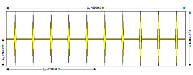
The general horizontal multifrac model is a homogeneous, single-phase, rectangular reservoir model consisting of a horizontal wellbore and transverse fractures. The horizontal multifrac solution is created through superposition of individual infinite conductivity fracture solutions in space.

The reservoir dimensions and well position may be specified by the user, provided the entire wellbore and all fractures fit within the reservoir boundaries. In addition, each fracture can be situated anywhere along the horizontal wellbore and configured to have a unique fracture half-length and conductivity. Thus, it is possible to model the combined effects of the horizontal wellbore and multiple fractures as well as the transition into middle-time flow regimes and boundary dominated flow for any number of different geometrical configurations. Depending on the configuration, pseudo-radial flow can be observed with this model.

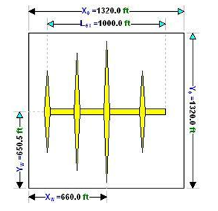
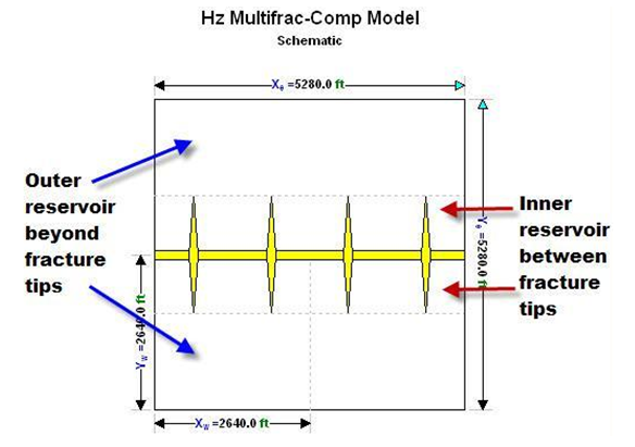
To specify fracture locations, half-lengths and conductivity a table is provided with each row representing one fracture in the model. The fracture location is specified as a X_w in relation to the center point of the horizontal well: a negative location represents a fracture to the left of the horizontal well center and a positive location is to the right.

Damage skin is applied along the length of the horizontal wellbore and a turbulence factor may be specified.

Horizontal Multifrac

Composite Model

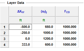
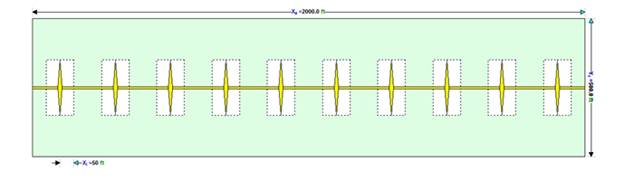
The horizontal multifrac composite model is a rectangular model that contains a non-contributing horizontal well fed by multiple identical and equally-spaced transverse fractures. The portion of the reservoir between the horizontal wellbore and the fracture tips is defined as the inner-reservoir and the rest is the outer-reservoir, as illustrated in the figure below. The permeabilities of the inner and outer regions can differ, making this model useful for modeling a stimulated reservoir volume (SRV) created by hydraulic fracturing which is fed by an unstimulated outer region.

This model calculates the reservoir's response from early-time storage and fracture flow, through the transition into boundary dominated flow. The fundamental building block of this model is the tri-linear fracture model for a vertical well. The outer-reservoir feeds the inner-reservoir via linear flow, the inner-reservoir feeds the fractures via linear flow, and the fluid within the fractures travels linearly towards the wellbore. However, for a horizontal well, the fluid within transverse vertical fractures actually has a radial flow pattern and a convergence skin has been implemented in order to account for this. As a result, it is not possible to observe radial flow with this model.

Note: A detailed description of the model is given by Brown et al. (2009)¹.

The reservoir dimensions, number of fractures and fracture half-length may be specified by the user, provided that the entire wellbore and all fractures fit within the reservoir boundaries. The dimensionless fracture conductivity must also be specified. A turbulence factor (D) can also be specified.

Horizontal Multifrac

SRV (Uniform Fracs) Model

This model is the same as the horizontal multifrac composite model, but includes only the inner region of the reservoir—not the outer reservoir region. In this model, fracture tips always extend to the edge of the reservoir.

Horizontal Multifrac

Enhanced Fracture Region Model

This model is a rectangular reservoir model consisting of a non-contributing horizontal well and transverse fractures. This model assumes that all the fractures are uniformly spaced with equal half-fracture length. (The reservoir can extend beyond the fracture tips.) This model has an improved effective permeability region around each fracture, and the distance from the fracture to the permeability boundary (X_I) can be specified by the user.

This model takes the following linear flow regimes into account:

linear flow within the fracture (at very early time)
linear flow within the stimulated region towards the fractures
linear flow within the non-stimulated regions towards the stimulated region
linear flow within the non-stimulated region towards the wellbore

Note: A detailed description of the model is given by Stalgorova and Mattar (2012)².

Analytical Model Parameters

Common Parameters

The following parameters appear in most or all analytical models

OGR	Oil-gas ratio
WGR	Water-gas ratio
p_i	Initial pressure
s	Skin (may be left blank)
h	Net pay
_t	Total porosity
S_g	Gas saturation
S_o	Oil saturation
S_w	Water saturation
c_f	Formation compressibility
X_e	Reservoir length
Y_e	Reservoir width
X_w	X position of well within reservoir
Y_w	Y position of well within reservoir (for horizontal well this is the middle of the horizontal length)
Z_w	Z position of the well within the reservoir net pay
r_w	Wellbore radius
D	Turbulence factor (may be left blank)
C_D	Storage coefficient (may be left blank)
OGIP	Original gas in place
OGIP_F	Original free gas in place
OGIP_A	Original adsorbed gas in place
A	Area, extent of reservoir

Model Specific Parameters

The following parameters are found in specific models. Models listed in right column

k	Permeability (all directions assumed to be the same)	Vertical, Fracture, Composite, Hz Multifrac Uniform
x_f	Fracture half-length	Fracture
(x_f)_y	Fracture half-length in y-direction	All Hz Multifrac models
F_CD	Fracture conductivity	All Hz Multifrac models
L_e	Effective horizontal well length	Horizontal
L_ex	Effective horizontal well length in x-direction	All Hz Multifrac models
k_x	Permeability in x-direction	Horizontal, Hz Multifrac
k_y	Permeability in y-direction	Horizontal, Hz Multifrac
k_z	Permeability in z-direction	Horizontal, Hz Multifrac
k_y/k_x	Ratio of y-direction to x-direction permeability	Horizontal, Hz Multifrac
k_z/k_x	Ratio of z-direction to x-direction permeability	Horizontal, Hz Multifrac
Perm ratios	Selecting this option allows the user to specify ratio values in place of k_y and k_z	Horizontal, Hz Multifrac
k1	Inner zone permeability	Hz Multifrac Composite, Hz Multifrac ERF
k2	Outer zone permeability	Hz Multifrac Composite, Hz Multifrac ERF
n_f	Number of fractures	All Hz Multifrac models
X_I	Distance from fracture to permeability boundary	Hz Multifrac ERF
r	Region radius	Composite
OGIP_SRV	Original gas in place in stimulated reservoir volume	Hz Multifrac ERF
A_SRV	Area of stimulated reservoir volume	Hz Multifrac ERF

1. Brown, M., Ozkan, E., Raghavan, R. and Kazemi, H. “Practical Solutions for Pressure Transient Responses of Fractured Horizontal Wells in Unconventional Reservoirs. SPE Paper 125043 prepared for Presentation at the 2009 SPE Annual Technical Conference and Exhibition, New Orleans, Louisiana. October 2009.

2. Stalgorova, E. and Mattar, L. “Practical Analytical Model to Simulate Production of Horizontal Wells with Branch Fractures. SPE Paper 162515 prepared for Presentation at the 2012 SPE Canadian Unconventional Resources Conference, Calgary, Alberta. October 2012.

Sandface C,n Deliverability

General

This deliverability option allows the user to specify the constants of the backpressure equation (also known as the Rawlins-Schellhardt equation), the Sandface "C" and the Sandface "n", to define the deliverability of the well at the sandface. The C and n value are generally determined from standard AOF/Back Pressure/Deliverability tests, but they can also be calculated/estimated from current operating conditions if some assumptions are made. This section will explain the various alternatives available to users.

When the Sandface Deliverability option is selected in the Well Deliverability editor, the information that defines the deliverability for that well is entered in the Wellbore Tuning editor. The Wellbore Tuning editor is accessible from the "Wells" menu option or using the Wellbore Tuning icon .

The Sandface C,n deliverability option uses the backpressure equation to define the wells deliverability. The backpressure equation is an empirically derived industry standard that applies to all gas wells, independent of reservoir drive. It is generally derived from AOF or Inflow performance testing. For Sandface Deliverability the backpressure equation is stated as:

Where:

q = flow rate, MMscfd or 103m3/d
C = constant, MMscfd/(psi2)n or (103m3/d/kPa2)n
n = turbulence of flow, dimensionless
PR = reservoir pressure, psi or kPaa
Pf = bottomhole flowing pressure, psi or kPaa

Sandface, C

The “C” value defines the magnitude of the wells rate response to changes in pressure. There are no limits on the range of allowed "C" values. Be aware however, the system is very sensitive to changes in "C" and that extreme values of "C" can result in extremely large deliverability potentials which can cause system instabilities.

Sandface, n

The inverse slope on the backpressure plot, "n", describes the effect of turbulence in the near wellbore region. Wells that are operating at high drawdowns, or wells with high permeability, can experience significant energy loss in the near wellbore region due to the development of turbulent flow from the high gas velocities. The “n” value helps account for this effect.

An "n" value equal to 1 describes completely laminar flow (no turbulence) and an "n" equal to 0.5 describes a very turbulent flow. In practice, values equal to 1 or 0.5 are not seen, but it is fairly common industry practice to use an n of 1 on low to mid deliverability gas wells that are not expected to operate at low drawdowns, and thus where turbulent effects will be minimal.

Values of n closer to 0.5 are most appropriate for wells that are expected to flow at high drawdowns, or for wells with high deliverability potential. Values approaching 1 are most appropriate for aging wells or for low deliverability wells. While in theory a value of n = 1 should not be possible, standard practice often prescribes an n value of 1 to aging or low deliverability wells that are expected to flow at a low rate.

Another common rule of thumb for n when it is not known is as follows:

<1 MMcfd use n = 1.0
>5 MMcfd use n = 0.5
1-5 MMcfd use n = 1.0 - 0.5 (interpolation)

This rule of thumb is simply an estimate. Many assumptions are being implicitly made when you follow the rule for defining an unknown n value. The n value is a function of permeability, or wellbore radius, of skin in the near wellbore region, and other variables, so making an assumption based purely on well rate needs to be understood in this context. If possible it is always better to use an n derived from a well test, or even from analogy of similar performing wells from the same geological structure.

The n value cannot be less then 0.5 or greater then 1.0. Input values less than 0.5 are automatically defaulted to 0.5 upon choosing OK to close the Well Deliverability Editor. Similarly, values greater than 1.0 are automatically defaulted to 1.0.

Using Turner or Coleman Correlation with Sandface Deliverability Wells

When the Turner or Coleman critical liquid lift correlations are turned on and a Sandface well has been selected, Piper will test for liquid loading and, if it is determined that the well cannot lift liquids through some or all of the wellbore, a pressure drop due to the existence of liquids in the wellbore will be applied.

Wellbore Tuning Editor for Sandface Deliverability Wells

The wellbore tuning editor in Piper allows you to tune the deliverability of a well and customize the well performance to the specific conditions that are being experienced in the field. The intent of the wellbore tuning editor is to allow you to:

Match well performance to existing conditions
Model reduced production levels (known as meta stable production), from liquid loaded wells
Forecast and estimate the impact of future liquid loading of a well
Estimate Sandface C for free flowing wells and liquid loaded wells

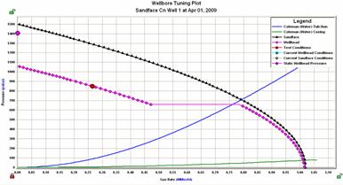
Understanding the Curves Being Displayed in the Wellbore Tuning Plot

The Wellbore Tuning plot displays the deliverability curves for the well, in addition to a few diagnostic curves.

Sandface Deliverability Curve: The Sandface Deliverability curve is the black curve, and it displays the pressure response at bottomhole as a function of well rate. The curvature is defined as per the C and n values entered by the user, while the Y-intercept is defined by the current reservoir pressure (when the flow rate equals zero).

Wellhead Deliverability Curve: The Wellhead Deliverability curve is the pink curve. The wellhead deliverability curve displays the pressure response at the wellhead as a function of well rate. The wellhead deliverability curve is determined from the sandface deliverability curve and the pressure losses in the wellbore. For any given rate, the Wellhead pressure can be defined as the Sandface pressure at that rate minus the pressure losses in the wellbore.

Liquid Loading Diagnostic for Casing: The blue and green parabolic shaped curves are the Liquid Loading diagnostics. There are two diagnostic curves displayed, one green and one blue. The green curve is a diagnostic for the casing. For any given pressure (measured at MPP) the green curve reflects the minimum flow rate required to lift liquids at MPP. For flow rates and pressures to the left of the green curve, liquids cannot be lifted at MPP, while for flow rates and pressures to the right of the green curve, liquids can be lifted at MPP.

Liquid Loading Diagnostic for Tubing or Annulus: The blue curve is the diagnostic for the tubing or annulus. For any given pressure (measured at EOT) the blue curve reflects the minimum flow rate required to lift liquids at EOT and above. For flow rates and pressures to the left of the blue curve, liquids cannot be lifted at EOT and above, while for flow rates and pressures to the right of the blue curve, liquids can be lifted at EOT and above.

The separate diagnostics for the tubing/annulus segment and the casing segment is because the diameter of each segment of the wellbore is different, and thus the same flow rate through both segments results in different velocities for the gas. Generally the tubing/annular segment is a smaller diameter then the casing segment, and thus a well will first reach a point where liquids cannot be lifted in the casing, followed at a later, lower rate by the point where liquids cannot be lifted in the tubing/annulus.

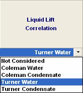
The user has the option to display either the Coleman or Turner diagnostic curves and to display either condensate or water as the primary fluid. The difference between choosing Coleman or Turner as your liquid lift diagnostic is explained in detail in the Turner and Coleman section.

Wellbore Tuning Plots when Liquid Lift is “Not Considered”

When the default Liquid Lift option is selected, liquid lift is “Not Considered” for the well. In this case Piper will not check to see if the well can or cannot lift liquids in the wellbore. The diagnostic curves may be drawn on the wellbore tuning plot, but will not be used internally by the program.

The result is that the Wellhead Deliverability curve is drawn throughout the range of pressures with the assumption that the single phase or multi-phase flow correlation being used is valid.

Wellbore Tuning Plot when a Liquid Lift Correlation is Selected

Description of Methodology

When the Turner or Coleman liquid lift correlation is turned on, Piper will take into account the ability of the wellbore to lift liquids. Piper will use the Turner or Coleman diagnostic to determine whether the gas rate is high enough at MPP and at EOT to carry liquids in the wellbore.

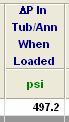
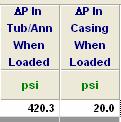
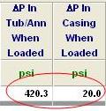
If the gas rate is not high enough at MPP to lift liquids in the casing, a pressure drop (specified in the “∆P in Casing when Loaded” cell) will be applied to the casing to account for the existence of liquids in that segment of the wellbore (from MPP to EOT).

The effect to the wellhead deliverability curve of adding the ∆P in the Casing is that the wellhead deliverability will undergo a step-change due to the extra pressure loss (see Figure below).

Note that the step change corresponds to where the Liquid Loading diagnostic curve for the casing (green) intersects the Sandface deliverability curve.

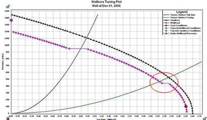
If the gas rate is not high enough at EOT to lift liquids in the tubing or annulus (depending on the flow path selected), a pressure drop (specified in the “∆P in Tub/Ann when Loaded” cell) will be applied to the tubing or annulus to account for the existence of liquids in that segment of the wellbore (from EOT to surface).

The effect to the wellhead deliverability curve of adding the ∆P in the Tubing or Annulus is that the wellhead deliverability will undergo a step-change due to the extra pressure loss (see Figure below).

Note that the step change corresponds approximately to where the Liquid Loading diagnostic curve for the tubing/annulus (blue) intersects the Sandface deliverability curve. Note that the two curves will not intersect at the exact point because the diagnostic is being compared at EOT, so the comparison will be a little bit off of the intersection, which would be if the comparison was being done at MPP.

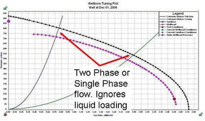
Modeling Wells that Produce at a Reduced Rate after Loading

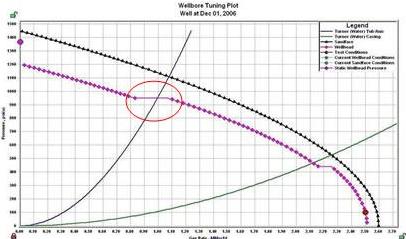
A well that flows at a reduced rate due to a step change in wellhead deliverability that is brought on by the onset of loading (and thus an accumulation of liquids in the wellbore) is said to be flowing at a meta-stable flow rate. There is evidence that in practice many wells flow at a meta-stable rate after loading occurs.

The concept of a meta-stable flow rate is used by Piper to describe the flow rate that a well will flow at after passing the onset of liquid loading, and thus having liquids existing in the wellbore.

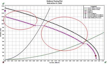
To illustrate the concept of a meta-stable flow rate, refer to the above figure. In the figure the wellhead deliverability curve is exhibiting two steps changes, one that illustrates the effect of liquids accumulating in the casing segment, and one that illustrates the effect of liquids accumulating in the tubing/annulus segment.

The flow rates along the wellhead deliverability curve that is circled and is just to the left of where the well loads in the casing are meta-stable flow rates with the casing loaded.

Similarly, flow rates along the wellhead deliverability curve that is circled and is just to the left of where the well loads in the tubing/annulus are meta-stable flow rates with the tubing/annulus is loaded.

Modeling a Well that is Expected to Shut-in after Loading

Note that if a well is expected to shut-in after loading in the tubing/annulus, the pressure specified in the “∆P in Tub/Ann when Loaded” can be adjusted to a high enough value that it overcomes the reservoir pressure, thus shutting in the well.

Modeling a Well that Produces Intermittently after Loading

After loading with liquids, many wells begin to produce in an intermittent fashion. Sometimes the well is shut-in for periods of time to help ‘re-energize’ the reservoir and blow out the liquids upon the commencement of flow. At other times, artificial lift techniques like plunger lift are used to unload the well, causing a fluctuating rate versus time behavior.

All of these scenarios describe situations where the well is undergoing a changing transient response over time. While the detailed, minute by minute response of the well is beyond the modeling scope of Piper, the concept a meta-stable flow rate can be applied to approximate the average behavior of such a well over a sufficient forecast period (the monthly forecast).

What needs to be determined is the average rate that the well would be expected to flow at after loading with liquids. For a well that has already loaded with liquids, this average rate is simply the current average production for that well. The current pressure is the average of the flowing pressure for that period.

To have the wellhead deliverability curve (pink) to align with the operating point, the pressure applied in the tubing/annulus segment, in other world the “∆P in Tub/Ann when Loaded” cell, can be adjusted to match up with the operating point (note that this can also be done using the “Auto-Match” button).

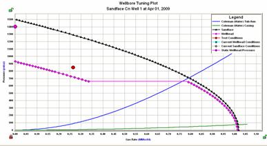
The resultant Wellbore Tuning plot will look something like the following figure:

The current operating point is the red circle. Note that, as you would expect, the wellhead deliverability curve runs through the current operating point. The response of this model is that the well will flow at the reduced average rate for the current period. Because the flow rate for the well is a function of the wellhead pressure, that flow rate will change as the wellhead pressure is increased or decreased. If the pressure can be reduced to a pressure where the well can again lift liquids in the tubing/annulus segment, the well will flow at a higher rate as it will unload in the tubing/annulus.

Its important to note the assumptions that are being made with this deliverability model.

What is essentially a transient response (be that plunger lift, manual shut-in, or natural reservoir shut-ins) is being approximated by the equivalent average pseudo-steady state response. If this transient response changes over time (the operating begins shutting in the well more frequently, the plunger lift cycle is extended or reduced), this will not be reflected in the model
The rate versus pressure response of the well assumes that the effect of the liquids (as defined by the “∆P in Tub/Ann when Loaded” that is specified) is independent of rate and pressure. The same ∆P is being applied to the tubing/annulus segment if the wellhead pressure goes up or down. This may only be an approximate assumption. For example, if this model is used on a well on plunger lift, the actual well response to increased tubing pressure would be a longer shut-in period, a shorter flow period, in other words a number of variables that may not exactly align with the response of the model.

With these assumptions being considered, the model still provides a good, albeit rough, approximation of well behavior after the well begins to load with liquids.

Description of Inputs Liquid Loaded Wells

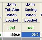
“∆P when Tubing/Annulus is Loaded” Selection

The “∆P in Tub/Ann when Loaded” cell is located towards the right hand side of the wellbore tuning editor.

The cell will be blue (not used in any calculations) when a Liquid Lift Correlation is “Not Considered”.

The cell will be white (considered in calculations and editable by the user) when a Liquid Lift Correlation is toggled on.

The value specified in the “∆P in Tub/Ann when Loaded” represents the pressure loss that is going to be applied to the tubing or annulus (depending on the flow path selected) when the well can no longer lift liquids at the EOT.

Note that once a well can no longer lift liquids at EOT, the only pressure loss applied to that segment will be the “∆P in Tub/Ann when Loaded”. There is no consideration made for frictional or hydrostatic losses due to flow above the liquid column. This is done to keep the model simple, and because the actual height of the liquids is both unknown and often times fluctuating over time.

“∆P when Casing is Loaded” Selection

The “∆P in Casing when Loaded” cell is located towards the right hand side of the wellbore tuning editor.

The cell will be blue (not used in any calculations) when a Liquid Lift Correlation is “Not Considered”.

The cell will be white (considered in calculations and editable by the user) when a Liquid Lift Correlation is toggled on.

The value specified in the “∆P in Casing when Loaded” represents the pressure loss that is going to be applied to the Casing segment (the flow path between EOT and MPP) when the well can no longer lift liquids at MPP.

Note that once a well can no longer lift liquids at MPP, the pressure loss specified in the “∆P in Casing when Loaded” cell will be the only pressure loss applied to that segment. There is no consideration made for frictional or hydrostatic losses due to flow above the liquid column. This is done to keep the model simple, and because the actual height of the liquid column is both unknown and often times fluctuating over time.

∆P Auto-Match

The “∆P Auto-Match” is located on the right hand side of the Wellbore Tuning editor.

The auto-match is only used for wells that cannot lift liquids. The auto-match can be used to automatically align the wellhead deliverability curve with the current operating point. This is accomplished by adjusting either the “∆P in Casing when Loaded” or “∆P in Tub/Ann when Loaded” values. The former is adjusted when the well cannot lift liquids at MPP but can at EOT. The latter is adjusted when the well cannot lift liquids at either MPP or EOT.

If the well can lift liquids throughout the wellbore, pressing the “∆P Auto-Match” will have no effect.

The “∆P Auto-Match” should only be used when the “Advanced” option is selected for a well.

To demonstrate the effect of pressing the “∆P Auto-Match”, consider the following case.

A well has its current operating point entered. A C,n value has been entered to define the deliverability. Initially, the operating point does not align with the wellhead deliverability curve.

A default value has been applied by the program to the “∆P in Tub/Ann when Loaded”.

Once the “∆P Auto-Match” Match button is pressed, the wellhead deliverability curve is aligned to fit the current operating point.

The value specified in the “∆P in Tub/Ann when Loaded” cell is changed to reflect the pressure drop required to make the wellhead deliverability curve align with the operating point.

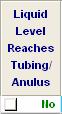
Liquid Level Reaches Tubing or Annulus

The “Liquid Level Reaches Tubing or Annulus” toggle allows the user to differentiate between wells where liquids will accumulate in the tubing or annulus and wells where the liquid level will not reach the tubing or annulus even if the well cannot lift liquids in the tubing/annular segment.

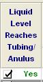
The specific situation that the “Liquid Level Reaches Tubing/Annulus” option is designed to account for is the situation where the tubing of the well is landed well above the perforations. If the tubing is well above MPP it is possible that liquids will accumulate in the wellbore to a level that is below the end of tubing, in which case even if the well cannot lift liquids above EOT, there is no additional liquids that accumulate.

The following criteria define the well performance after the tubing or annulus can no longer lift liquids:

When the Liquid Level If the “Liquid Level Reaches Tubing/Annulus” check box is toggled, the pressure drop specified in the “∆P in Tub/Ann when Loaded” cell will be applied to the wellbore Tubing/Annulus segment.
If the “Liquid Level Reaches Tubing/Annulus” check box is not toggled, single phase flow will be assumed in the Tubing/Annulus segment.

Description of Methods that can be Used to Model Behavior when Well Loads (Method Used when Well Loads column)

The “Method Used when Well Loads” options are available (in white) after a Liquids Lift Correlation has been selected, and thus when liquid loading is considered for the well. If the Liquid Lift Correlation is not considered, the cell will remain blue and not be used in any calculations.

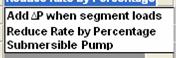
There are 3 options that can be selected from when a well loads with liquids. These options are:

Add ∆P when Segment Loads
Reduce Rate by Percentage
Submersible Pump

Each method will treat the well somewhat differently once the well cannot lift liquids at MPP or EOT.

Add ∆P when Segment Loads

With the “∆P when Segment Loads” option, both the “∆P in Tub/Ann when Loaded” and the “∆P in Casing when Loaded” cells will be available and used in the calculations.

When the “∆P when Segment Loads” option is selected, the following criteria will apply:

· When the well cannot lift liquids at MPP (as determined by the selected Liquid Lift Correlation), the pressure drop specified in the “∆P in Casing when Loaded” cell will be applied to the wellbore casing segment.

· When the well cannot lift liquids at EOT (as determined by the selected Liquid Lift Correlation), the criteria depends on whether the “Liquid Level Reaches Tubing/Annulus” option is toggled on or off.

o If the “Liquid Level Reaches Tubing/Annulus” check box is toggled, the pressure drop specified in the “∆P in Tub/Ann when Loaded” cell will be applied to the wellbore Tubing/Annulus segment.

o If the “Liquid Level Reaches Tubing/Annulus” check box is not toggled, single phase flow will be assumed in the Tubing/Annulus segment.

Reduce Rate by Percentage

With the “Reduce Rate by Percentage” option, only the “∆P in Casing when Loaded” cell is available and editable. An additional cell, in the “Percent Reduction in Rate” column, is editable.

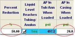
The following criteria will be applied when the “Reduce Rate by Percentage” option is chosen:

· When the well cannot lift liquids at EOT (as determined by the selected Liquid Lift Correlation), the well rate at the onset of loading is reduced by the percentage specified.

Note that for this option, a value will be populated in the blue cell “∆P in Tub/Ann when Loaded”. This value is not editable. It is calculated by Piper and is the pressure drop that must be applied to the tubing to satisfy the percent rate reduction that has been specified. Internally Piper is using this value to come up with the rate reduction that is anticipated.

Submersible Pump

With the “Submersible Pump” option, the “Fluid Column Height”, “Fluid Column GLG” and the “∆P in Casing when Loaded” cells are available and editable.

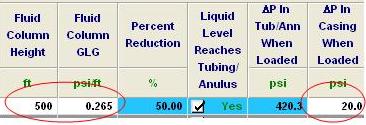
The following criteria will be applied when the “Submersible Pump” option is chosen:

· When the well cannot lift liquids at EOT (as determined by the selected Liquid Lift Correlation), a submersible pump will be assumed to be installed at EOT.

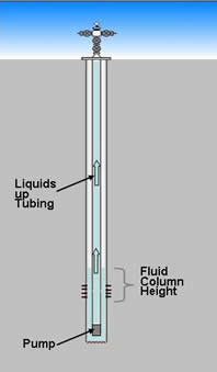
· Liquid flow is up the pump through the tubular side (see figure)

· Gas flows on the annular side (see figure)

· A liquid column of the gradient and height specified is applied. Note that the liquid column height is defined from MPP.

· Above the liquid column, in the annulus, single phase gas flow is assumed.

Submersible Pump

Determining Sandface C For Sandface Deliverability Wells

If current wellbore and flowing conditions for a well are known, the Sandface Deliverability of a well can be calculated. While not as reliable as a deliverability estimate from a welltest (where a number of flowing conditions, rather then a single condition, are used to calculate deliverability), the estimate can still be used to approximate how pressure versus rate response of the well over time.

The Sandface C button will initiate a calculation of Sandface Deliverability for the selected well. The Sandface C button is located in the upper left portion of the Wellbore Tuning plot.

Sandface C can be calculated using flowing pressures or using non-flowing pressures. For loaded wells, calculations of Sandface C using flowing pressures are unreliable and non-flowing pressures should be used when available.

Caution when using the Sandface C Button

When a well can lift liquids throughout the wellbore, the calculation of Sandface C using flowing pressures can be quite reliable. When the well cannot lift liquids within the wellbore the calculation of Sandface C becomes less reliable if flowing pressures are used to calculate the current bottomhole pressure.

If a well cannot lift liquids in the casing segment (at MPP) usually the calculation of Sandface C using flowing pressure is usually still reasonably reflective of the actual well behavior. This is because generally the tubing is landed close to MPP, and thus the accumulation of liquids in the casing results in a minimal pressure drop.

On the other hand, the calculation of Sandface C using flowing pressures for a well that has liquids accumulating in the tubing is much less relaible. The uncertainty about the height of the liquid column can lead to large errors.

Calculating Sandface C using flowing pressures for a well that cannot lift liquids in the tubing/annulus segment should be recognized as only an estimate of Sandface Deliverability and should be interpreted as such. When a well cannot lift liquids in the tubing it is preferable to either calculate Sandface C from non-flowing pressure data, or to

Inputs for the Calculation of Sandface C

Before Piper can calculate the value of Sandface C for a well, the user must input a number of parameters defining both the current well performance as well as the wellbore.

The minimum inputs that need to be defined by the user are:

A Surface Test Conditions: as defined by the Surface Test Rate, Surface Test Pressure (Tubing and/or Casing) and LGR

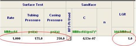
Note that if flowing pressure is going to be used to calculate Sandface C, only the flowing pressure (either tubing or casing) needs to be specified. If non-flowing pressure is going to be used, both tubing and casing pressure needs to be specified.

Wellbore and Flow Path

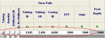
Note that if the MPP is not specified, it will be assumed to be the same as the pool depth. If the EOT is not specified it will be assumed to be the same as MPP.

Pressure Loss Correlation

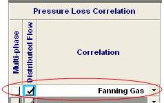
The Multi-phase flow option is selected if liquids exist in the well. If Beggs and Brill is used, the distributed flow option can be toggled if the user wants to “force” the distributed flow regime in the wellbore.

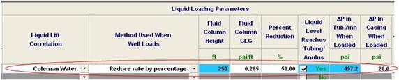
If the user wants to consider the ability of the well to lift liquids, these options can be accessed under “Liquid Loading Parameters”

Status of Turner and Coleman critical liquid lift tests

The Sandface C Calculation

Calculation of Sandface C for Wells where Liquid Loading is not Considered:

If neither the Turner or Coleman critical liquid lift tests are selected, Piper will not take into consideration the ability of the well to lift liquids in its calculation of Sandface C.

Piper will assume that the gas can lift liquids throughout the wellbore. The single phase or multi-phase correlation will be applied to the length of the wellbore.

A value for Sandface C will be calculated based on the current flowing pressure, rate and LGR that have been entered as the Surface Test condition.

The above figure illustrates how the ability of the well to lift liquids is ignored. Note that to the left of the liquid loading diagnostic curves for the tubing/annulus and casing (blue and green curves) there has been no change to the wellhead deliverability curve.

Calculation of Sandface C Using Non-Flowing Pressure for Wells that Consider Liquid Loading

Piper can estimate the Sandface Deliverability of a well that can no longer lift liquids by using the non-flowing pressure.

Note that non-flowing pressure can only be used when a well does not have a packer installed downhole.

Theory Behind using Non-flowing Side Pressures to Calculate Well Deliverability

The application of non-flowing pressure to calculate Sandface C comes about because of the unreliability of using flowing side pressures for wells that cannot lift liquids in the tubing/annulus. The extent that liquids accumulate in the tubing/annulus is an unknown, and therefore using flowing side surface pressures to estimate bottomhole conditions is unreliable. On the other hand, with non-flowing side pressures, a much more reliable bottomhole pressure estimate can be attained.

The theory behind using non-flowing pressures to calculate Sandface C is based on the distribution of liquids in a wellbore once a well can no longer lift liquids to surface.

Consider the scenario where a well can no longer lift liquids to surface either in the casing or the tubing. Liquids will accumulate in the wellbore in both segments of the wellbore (see figure below).

Note how the liquids accumulate on the flowing side of the wellbore (in this case in the tubing), but not on the non-flowing side (annular side).

Because liquids do not accumulate along the non-flowing side, the only pressure drop across that side is due to the presence of the gas. The calculation of the pressure drop from surface to EOT due to the hydrostatic column of gas is a reliable one.

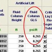
For most wells, the end of tubing is landed within a short distance of MPP. Thus the pressure drop in the casing segment due to the liquids that have built up is generally small in relation to the reservoir pressure, and therefore an approximation of this pressure drop is usually sufficient. In Piper, by default the assumption will be made that the pressure loss in the casing due to liquids is equal to the length of the casing segment (the distance from MPP to EOT) multiplied by a gasified liquid gradient of 0.265 psi/ft.

The gradient of 0.265 psi/ft is an experienced based estimate of the effect of accumulated liquids in the wellbore. The overall effect of liquids on the casing segment can be modified by the user by changing the value of the “∆P in Casing when Loaded” cell.

F.A..S.T Piper will thus calculate the pressure at the Sandface using a combination of the gas gradient down the non-flowing side, and an estimate of the pressure drop due to the liquids that have accumulated from EOT to MPP.

Once a pressure loss at the Sandface is calculated, it is a relatively simple calculation of C. In addition, Piper will calculate what the pressure drop due to accumulated liquids along the flowing side must be to satisfy the fact that the pressure and EOT is equal on both the flowing and non-flowing side. The calculated pressure drop on the flowing side is then input in to the ∆P in Tub/Ann when Loaded cell.

Input Requirements to Perform the Calculation of Sandface C using Non-flowing side Pressure

The calculation of Sandface using non-flowing side pressures can be performed whenever a Liquid Lift Correlation has been selected:

The use of non-flowing side pressures to calculate Sandface C requires that the “Use Non-Flowing Pressure Data” option be toggled.

Calculation of Sandface C Using Flowing Pressure for Wells that Consider Liquid Loading

As already noted, when the well cannot lift liquids within the wellbore the calculation of Sandface C using flowing pressure data becomes less reliable. This is due to the existence of accumulated liquids along the flowing side, and the lack of information available to accurately define the effect of those liquids on the overall wellbore pressure drop (in particular the liquid height is generally unknown, and the gradient can only be estimated).

It is important here to distinguish again between a well that cannot lift liquids in the casing, and one that cannot lift liquids in the tubing. If a well cannot lift liquids in the casing segment (at MPP) the calculation of Sandface C using flowing pressure data usually still reasonably reflects the actual well behavior. This is because generally the tubing is landed close to MPP, and thus the accumulation of liquids in the casing segment of the wellbore has a minimal effect on the overall pressure drop.

On the other hand, the calculation of Sandface C using flowing pressures for a well that has liquids accumulating in the tubing is much less reliable. The uncertainty about the height of the liquid column can lead to large errors.

Piper provides the functionality to estimate a value of Sandface C from a loaded well while using flowing pressures. There are actually two estimates of C that Piper can make, and these two estimates can be considered to bound the range of possible solutions with the most optimistic deliverability possible, and the most pessimistic deliverability possible. While neither estimate will likely reflect the actual deliverability of the well, these estimates can be used, along with historical decline data, to come up with a C value that both forecast the well production forward so that it matches that historical decline, and that predicts an unloaded condition that matches the expected rate if the well was unloaded.

Optimistic Deliverability Estimate

The Optimistic Deliverability estimate is attained by setting the “Liquid Level Reaches Tubing/Annulus toggle to “Yes” before calculating Sandface C for the well.

Piper will assume that:

If the wellhead pressure could be reduced 1psi, the well would unload in the tubing.

The most optimistic deliverability possible for a loaded well will occur if that well is just on the cusp of loading. The result of this optimistic estimate is the largest value of Sandface C (and therefore the largest AOF) possible for that well given its current flow rate and wellbore definition.

Pessimistic Deliverability Estimate

The Pessimistic Deliverability estimate is attained by setting the “Liquid Level Reaches Tubing/Annulus” toggle to “No” before calculating Sandface C for the well.

Piper will assume that:

In the wells current state, while liquids cannot be lifted in the tubing/annulus there are no liquids that have accumulated in the tubing/annulus

The most pessimistic deliverability possible for a loaded well will occur if, though loaded, liquids have not accumulated in the tubing of that well. The result of this pessimistic estimate is the smallest value of Sandface C (and therefore the smallest AOF) possible for that well given its current flow rate and wellbore definition.

Pumping Flow Path

Users have the option to specify that a well is currently pumping and therefore use artificial lift as the flow path. The artificial lift scenario that Piper will simulate is a submersible pump located at EOT. In such a scenario, the pump is assumed to produce the liquids up the tubing, while gas is produced up the annulus.

The fluid filling the Fluid Column Height in the annulus of the wellbore is assumed to be of a gradient equal to the Fluid Column GLG.

When artificial lift has been selected, Piper will calculate the pressure loss in the wellbore based on the assumption that liquids exist up to some level in the annulus, and that beyond that liquid level single phase gas flows.

When EOT is above MPP then the pressure drop due to the liquid column in the annulus will include the height of the fluid column from MPP to EOT. When EOT is below MPP, then the pressure drop due to the liquid column in the annulus will use the height of the fluid column less the distance from end of tubing to the midpoint of perforations.

The gasified liquid gradient for all segments of the wellbore loaded with liquids is defined by the value of the Fluid Column GLG.

No Wellbore

No wellbore is a special case of artificial lift where the impact of the liquid column in the annulus and the frictional effect of gas traveling up the wellbore are ignored. Piper thus uses only a static gas gradient from the reservoir to surface.

No Wellbore is the default option for transient wells that have been imported from previous versions of Piper.

Turner and Coleman Critical Liquid Lift Correlations

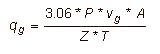
When gas production is associated with water or condensate production, a minimum gas flow rate required to lift liquids has to be determined at a given flowing pressure, temperature and tubing diameter.

R. G. Turner, M. G. Hubbard and A. E Dukler first presented the Turner critical liquid lift correlation at the SPE Gas Technology Symposium held in Omaha, Nebraska, September 12 and 13, 1968. The correlation (SPE paper 2198) calculates the minimum gas flow rate required to lift liquids out of a wellbore and is often referred to as The Liquid Lift Equation or Critical Flow Rate Calculation for Lifting Liquids.

Steve B. Coleman, Hartley Clay, David McCurdy and Lee Norris published a series of papers dealing with the phenomena of liquid loading. The papers presented a modified version of the Turner correlation that appeared to agree more closely with real life liquid loading data.

Piper uses the Turner and Coleman critical liquid lift correlations to determine when the onset of liquid loading in the wellbore will occur.

The Turner and Coleman diagnostic curves can be displayed in the wellbore tuning plot. Piper will display the curve for the Tubing / Annulus segment of the wellbore (the critical liquid lift calculation is performed at the end of tubing) and for the Casing segment (the critical liquid lift calculation is performed at the mid point of perforations).

The curves can be displayed for either water or condensate, whichever is the dominant fluid in the wellbore.

The Turner and Coleman critical liquid lift correlations need to be activated before they will be used to determine the state of loading in the wellbore. Activation occurs when water or condensate box is checked for either correlation.

Use of the Turner and Coleman Critical Liquid Lift correlation can be activated in 3 possible menus, depending on the type of well:

Wellbore Descriptions Menu:activates correlation for Transient and Sandface wells
Wellbore Tuning Menu:activates correlation for Sandface wells

Theory of Turner and Coleman Critical Liquid Lift Correlations

The Turner and Coleman correlations assume free flowing liquid in the wellbore form droplets suspended in the gas stream. Two forces act on these droplets. The first is the force of gravity pulling the droplets down and the second is drag force due to flowing gas pushing the droplets upward. If the velocity of the gas is sufficient, the drops are carried to surface. If not, they fall and accumulate in the wellbore.

The Turner correlation was developed from droplet theory. The theoretical calculations were then compared to field data and a 20% fudge factor was built-in. The correlation is generally very accurate and was formulated using easily obtained oilfield data. Consequently, it has been widely accepted in the petroleum industry. The model was verified to about 130 bbl/MMscf. The Turner correlation was formulated for free water production and free condensate production in the wellbore.

From the minimum gas velocity, the minimum gas flow rate required to lift free liquids can then be calculated using:

The Coleman correlation effectively removed the 20% factor that Turner had added to his correlation after finding that this provided better predictions for low pressure wells (less then 500psi). Apart from this, Coleman is using a methodology consistent with what Turner used.

How Equation of State affects Deliverability

All of the Piper well deliverability models are functional with the equation of state or equilibrium ratio model (either Peng-Robinson, Modified Wilson or Wilson).

When Peng-Robinson or one of the equilibrium ratio methods has been turned on, Piper will convert the gas and oil volumes defined by the deliverability relationship and OGR(or in the case of fixed rate and profile wells, the specified oil and gas rates) into an equivalent recombined molar rate. The molar rate is then flashed at the changing pressure and temperature conditions throughout the pipeline system in order to determine the gas and oil volumes.

Note that in the Wellbore Tuning plot and in deliverability plots, the gas rates shown are the recombined rate and do not reflect the actual in-situ gas rates flashed to by the equation of state or equilibrium ratio model.

Standard Rates and In-situ Rates

Both in-situ and standard rates can be displayed in the annotations of all nodes, wells and facilities, and in most facility plots.

In-situ Rates

In-situ rates are defined as the rate of each phase (gas, oil and water) present at the temperature and pressure of a given point in the system.

In black oil this means translating the standard condition volume of gas with the amount of gas in water (R_sw) and gas in oil (R_so) at the pipeline condition, and translating the volume of water in the gas (Water of condensation) at the pipeline condition.

For equation of state and equilibrium ratios this means the flashed oil and gas volumes at pipeline conditions.

It’s important to make the distinction that in-situ rates are still converted in plots and annotations to their equivalent standard condition volume. This is done to be consistent with the common practice to always display gas rate in MMscfd.

Standard rates

Standard rates are defined as the rate of each phase (gas, oil and water) present at standard conditions.

In the same manner as for in-situ rates, for black oil standard rates are determined by translating volumes using R_so, R_sw and water of condensation. Likewise, for equation of state and equilibrium ratios, standard rates are determined by flashing the rates at standard conditions.

Terminology

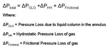
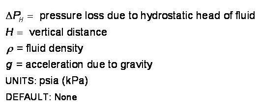
Hydrostatic Pressure Loss

This refers to a pressure loss caused by the weight of a vertical column of fluid. The equation for this relation is:

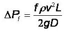
Frictional Pressure Loss

This refers to the pressure drop in a length of pipe that is caused by frictional effects. The governing equation for friction loss is:

EOT

End of tubing.

MPP

Mid point of perforations.

Liquid to Gas Ratio

Piper assumes that liquid production will follow in a constant ratio to gas production, known as the liquid to gas ratio. Multiplying the gas rate by the liquid to gas ratio will calculate the liquid production for the well.

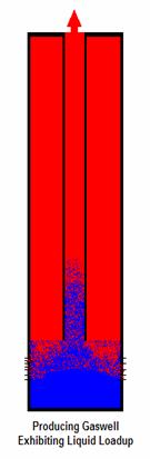
Liquid Loading

As natural gas is produced, the energy available to transport the produced fluids to surface declines. This transport energy eventually becomes low enough that flow rates are reduced and fluids produced with the gas are no longer carried to surface but are held up in the wellbore. These liquids accumulate in the wellbore over time, and cause additional hydrostatic back pressure. This phenomena is known as liquid loading.

Alias Name

The intent of the alias name is to provide another name for the well.

Minimum Gas Rate

Often the operating conditions of a well are such that below a certain rate, it is uneconomical or impractical to keep producing the well. This can be due to such factors as wellbore liquid load-up, or excessive operating costs like hydrate prevention, water disposal, etc. The minimum gas rate allows the user to set the rate at which a well will be shut-in. Once a well's flow rate falls below the Minimum Gas Rate, it is turned off and remains off.

Note: A well may prematurely fall below the Minimum Gas Rate if low contract rates cause the flow of all wells to be choked back. The user may choose to produce one well preferentially and delay the start of other wells until they are needed or set a minimum gas rate limit equal to 0 such that the well will come on-stream when the backpressure is low enough to commence production. Any well (regardless if a Minimum Gas Rate is specified or not) will be turned off if the rate drops below .005 MMscfd (0.14 103m3/d).

Maximum Gas Rate

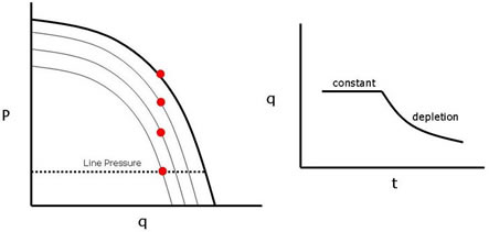
The Maximum Allowable Gas Rate is a restriction that is applied to a well's production rate such that the well is not allowed to produce above that rate. This limitation may be caused by government regulations (allowables, off-target penalties, etc.) or good production practice. As the well deliverability decreases, the drawdown on the well will increase until it is equal to the line pressure. At this point the well will follow normal depletion.

NOTE: The Maximum Allowable Gas Rate essentially acts in the same way as a contract restriction on an individual well. The difference is that Piper tracks the maximum deliverability potential which is calculated without contract restrictions but after the Maximum Allowable Gas Rate and Maximum Drawdown Limit restrictions are applied (any or all of the Maximum Allowable Gas Rate, Maximum Drawdown Limit and Minimum Rate can be applied to a well).

Maximum Drawdown Limit

For some wells, for example those wells that are experiencing water coning, it is desirable to impose a Maximum Drawdown Limit rather than a Maximum Rate. A commonly used value is 15 to 25%. Drawdown is defined as:

Drawdown = 100 x (shut-in pressure - flowing pressure)/shut-in pressure (%)

When a maximum drawdown is specified, the well will be choked back to a rate consistent with the pressure drawdown.

Note: The Maximum Drawdown Limit is expressed as a percentage but will result in a maximum rate limitation that decreases as the reservoir pressure decreases. This differs from the Maximum Rate option which remains fixed irrespective of reservoir pressure. The Maximum Drawdown Limit addresses reservoir management whereas the Maximum Rate handles surface or regulatory restrictions (any of all of the Maximum Rate, Maximum Drawdown Limit or Minimum Rate can be applied to a well).

Drawdown is calculated at the sandface if the Wellbore option is used. Otherwise, drawdown is calculated at the wellhead (the difference is significant only if you have high wellbore friction pressure losses i.e. a really good well).

UNITS : Percent (%)

DEFAULT : 100%

Surface Equipment Pressure Loss

For some wells, there is a restriction (for example a dehydrator, line heater, or riser) between the wellhead and the pipeline of the gathering system. The pressure drop across these vessels is handled as a fixed pressure drop (independent of rate).

UNITS: psia (kPaa)

DEFAULT: None

Measured Gas Line Pressure

The Measured Gas Line Pressure can be input and compared to the gas line pressure calculated by Piper. The difference between the measured gas line pressure and the calculated gas line pressure will be displayed in the bubble map menu when the Pipeline Pressure Calibration map type is selected.

Measured Water Line Pressure

The Measured Water Line Pressure can be input and compared to the gas line pressure calculated by Piper. The difference between the measured water line pressure and the calculated gas line pressure will be displayed in the bubble map menu when the Gas and Water Line Difference map type is selected.